


Advanced Lens Selection
This is Section 6.3 of the Imaging Resource Guide.
The prior section explained lens selection primarily from the perspective of the lens as the final component to be chosen in the machine vision system. This section approaches lens and camera selection holistically, choosing both at the same time, depending on what is important for the specific application. This section will walk through an example starting from scratch where a 2D barcode needs to be imaged from 200mm away, as shown in Figure 1.

Figure 1: Image of the 2D barcode that must be imaged from 200mm away.
Starting with the object to be inspected and breaking it down into its constituent parts is the first step in lens selection. What are the important features? How large are these features? How many pixels do I need to cover the feature that I am trying to observe in order for my machine vision software to function properly?
Often, the best place to start is feature size and pixel coverage. For the barcode in Figure 1, these are fairly straightforward numbers. The feature size is 100µm, with empty space of at least 100µm in between features. This means that the frequency that this feature corresponds to is 5$ \small{ \tfrac{\text{lp}}{\text{mm}}} $ (see Resolution for a review of this math) in object space. This number is the first piece of the puzzle in determining the required magnification of the lens.
Next, the entire field of view (FOV) needs to be considered. This means not only the size of the barcode itself, but space must be allowed for positional uncertainty within the FOV. If the barcode is 25mm x 25mm, it is likely safe to say that a FOV of 35mm is required. In this particular example, it is necessary to have at least three pixels covering each feature on the barcode. Since the feature size on the barcode is 100µm, it is then required to have at least 33µm per pixel on the object plane.
At this point, different cameras can be evaluated to see if it is possible to achieve this. In order to keep costs minimal, it can be important to start with as small a resolution as possible. In today’s machine vision world, this is often 0.3MP, or VGA resolution (640x480). Looking at the aspect ratio of the sensor, it is exactly 4:3. However, the FOV that is needed is 1:1; this means that the small dimension of the sensor (480 pixels) will need to be used to correspond to the 35mm FOV, and the larger dimension will float and there will likely be some wasted pixels.
Because 480 pixels are going to be divided among 35mm of space, each pixel corresponds to 110µm in object space. This camera is certainly insufficient for this application, and it is required to have a resolution about 3X better. Running through the math again with a 1600x1200 sensor with 4.5µm pixels, each pixel now takes up 29µm, which is sufficient. But how does this correspond to image space with a camera and lens? At this point, the system needs to be linked to the magnification.
Since this 1600 x 1200 sensor has pixels that correspond to 4.5µm in size, the dimensions are 7.2mm x 5.4 mm. Using Equation 4 in Basic Lens Selection, the magnification required is 0.15X. It is now possible to use this magnification to determine which lens is needed, as well as what the imaging system needs to be able to achieve from a resolution point of view in order to properly image the barcode. Since a sensor has been chosen, Equation 3 from Basic Lens Selection can now be used to determine the focal length of the lens. Using Equation 3, the focal length required based on the 200mm working distance (WD) is 30mm. However, the magnification required (0.15X) can be achieved with a 25mm lens from 230mm away; in this example this is sufficient. Now a preliminary lens has been chosen, but can it work based on the resolution required?
The resolution required in object space is 5$ \small{ \tfrac{\text{lp}}{\text{mm}}} $. Converting this into image space by dividing by the magnification, 33$ \small{ \tfrac{\text{lp}}{\text{mm}}} $ is required in order to view the object properly. This number needs to be checked against two numbers: the Nyquist frequency of the sensor, and the modulation transfer function (MTF) of the lens that is being used. See Resolution for more information on the Nyquist frequency. Equation 1 describes the Nyquist frequency of a sensor as:
Where s is the pixel size. Using Equation 1, a sensor with 4.5µm pixels has a Nyquist frequency of 111$ \small{ \tfrac{\text{lp}}{\text{mm}}} $. Because this is larger than the required 33$ \small{ \tfrac{\text{lp}}{\text{mm}}} $, this camera is a good choice. The astute reader may note that this will link back to the fact that we have three pixels covering our feature, and we are unsurprisingly at about 3X below the Nyquist frequency. This math was included here for completeness.
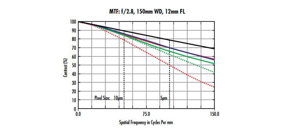
The MTF curve for a 25mm C Series Fixed Focal Length Lens from a WD of 166mm can be found in Figure 2 (for more information on how to read an MTF curve, see The Modulation Transfer Function). Looking at the curve, it can be seen that the 25mm lens achieves about 83% contrast at 33$ \small{ \tfrac{\text{lp}}{\text{mm}}} $, which is more than sufficient to image it well.

Figure 2: MTF curve of a 25mm C Series fixed focal length lens that achieves a more than sufficient resolution for this example.
As a general rule of thumb, a minimum contrast value that is required for an imaging lens to properly resolve an object is 20%, meaning that this lens has more than enough resolution to see this barcode sufficiently.
This is just the tip of the iceberg when selecting a lens for a given application. MTF is affected by several factors (explained in detail in MTF Curves and Lens Performance), and oftentimes it is not straightforward. The following section goes into detail on looking specifically at a lens and how well it matches to a camera.
The Changing Performance of a Lens
Lens suppliers are able to provide bespoke MTF curves based on how the lens is used. In the barcode example above, the MTF of the 25mm lens was referenced to determine if it had sufficient contrast reproduction for the barcode that it was imaging. Now, we will expand on this using a different example, but with the same lens, to show how things do not always work out as intended.
Figure 3 shows two different MTF curves of the same 25mm fixed focal length lens at the same WD (providing a magnification of 0.76X), but different f/#s and wavelength ranges. They hardly look like the same lens! The important takeaway is that just looking at MTF curves on specification sheets will not adequately explain the performance of a lens everywhere throughout its range, and specific curves are a necessity.


Figure 3: A high resolution 25mm lens’s MTF at different settings, reinforcing the importance of comparing the specific lens curves.
Based on the MTF of a given lens, the minimum resolvable feature size in object space can be determined. However, MTF curves are always in image space, which means the image space information must be transformed into object space information. Luckily, this is as simple as scaling by the magnification. The following example illustrates how to complete these calculations using the curves in Figure 3 as a starting point. Assuming a contrast minimum of 20% for this example, the lens on the top can resolve 250$ \small{ \tfrac{\text{lp}}{\text{mm}}} $ in image space, which is determined by finding the frequency on the curve that matches 20% contrast. Using Equation 2, the pixel size (or in this case, the image space resolution
$ \small{\xi _{\small{\text{Image Space}}}} $ converted from a frequency to a physical object) is calculated to be:
Scaling by the magnification (0.076X) results in:
In comparison, the lens with the curve on the bottom in Figure 3 can only confidently image an object that is 282µm in size (using the same math as the above example). The example on the previous page also assumes that the exact camera/sensor has not yet been chosen, therefore making the optics the limiting component in the imaging system. If a camera sensor had been chosen prior to the lens, the lens would need to be able to resolve the pixel size of the sensor in use.
Continuing from the example on the previous page, if a camera had been chosen with the Sony IMX250 sensor with 3.45µm pixels, using Equation 2 the image space resolution can be found as 144.9$ \small{ \tfrac{\text{lp}}{\text{mm}}} $. Looking at the MTF curve, the lens achieves >40% contrast, which is more than enough for most applications. However, using the same calculation as in Equation 3 to scale into object space, 3.45µm pixels only corresponds to a 45µm object, meaning the sensor would be the limiting component in the system, as the lens is capable of 26µm object space resolution. All of these considerations must be made when determining the proper lens for a given application in order to find the optimal solution to a machine vision problem.


or view regional numbers
QUOTE TOOL
enter stock numbers to begin
Copyright 2023 | Edmund Optics, Ltd Unit 1, Opus Avenue, Nether Poppleton, York, YO26 6BL, UK
California Consumer Privacy Acts (CCPA): Do Not Sell or Share My Personal Information
California Transparency in Supply Chains Act
This content may include material that has been generated or modified using artificial intelligence (AI).
The FUTURE Depends On Optics®